Introduction
Back-propagation has been the engine driving the deep learning revolution. We’ve come a long way with advancements such as:
- New layers like Convolutional Neural Networks, Recurrent Neural Networks, Transformers.
- New training paradigms like fine-tuning, transfer learning, self-supervised learning, contrastive learning, and reinforcement learning.
- New optimizers, regularizers, augmentations, loss functions, frameworks, and many more…
However, the Abstraction and Reasoning Corpus (ARC) dataset, created over five years ago, has withstood the test of numerous architectures but never budged. It has remained one of the toughest datasets where even the best models could not beat human level accuracies. This was an indication that true AGI is still far from our grasp.
Last week, a new paper “The Surprising Effectiveness of Test-Time Training for Abstract Reasoning” pushed a relatively novel technique forward, reaching a new state of the art level of accuracy on the ARC dataset that has excited the deep learning community akin to how AlexNet did 12 years ago.
TTT was invented five years ago, where training occurs on very few samples—usually one or two—similar to the testing data point. The model is allowed to update its parameters based on these examples, hyper-adapting it to only those data points.
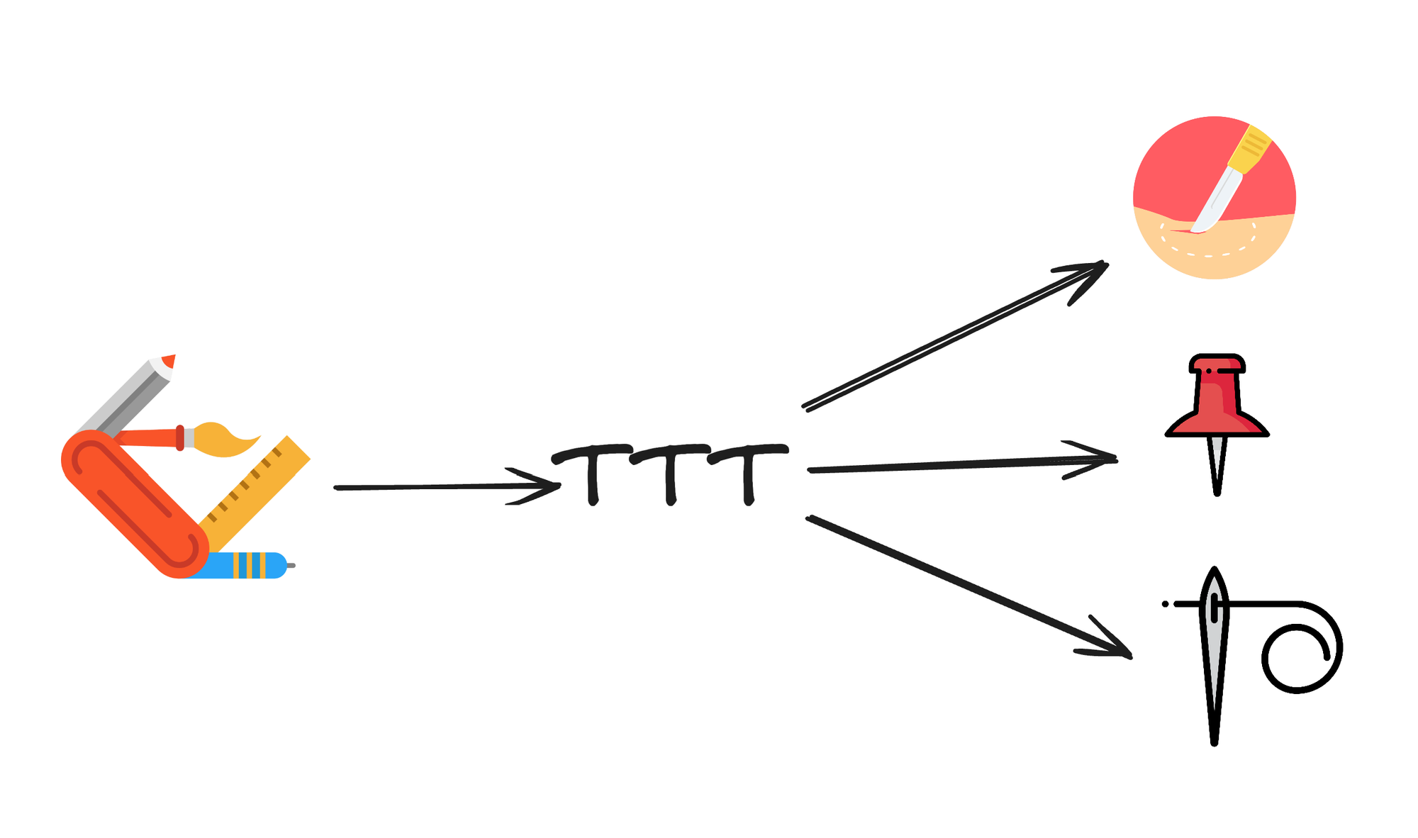
TTT is analogous to transforming a general physician into a surgeon who is now super specialized in only heart valve replacements.
In this post, we’ll learn what TTT is, how we can apply it in various tasks, and discuss the advantages, disadvantages, and implications of using TTT in real-world scenarios.
What is Test Time Training?
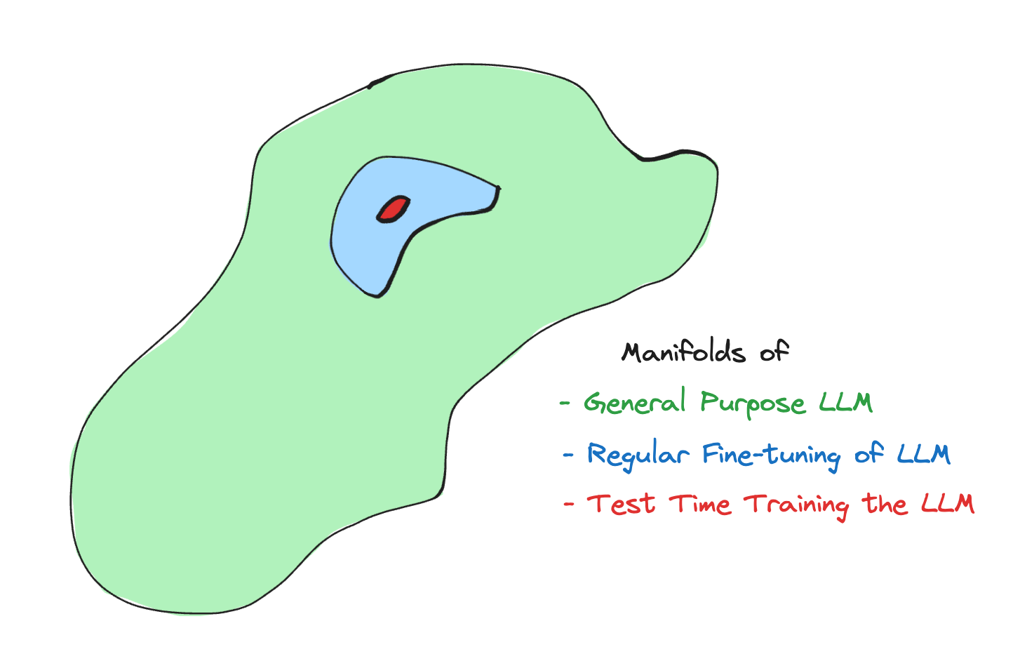
Humans are highly adaptable. They follow two learning phases for any task—a general learning phase that starts from birth, and a task-specific learning phase, often known as task orientation. Similarly, TTT complements pre-training and fine-tuning as a second phase of learning that occurs during inference.
Simply put, Test Time Training involves cloning a trained model during testing phase and fine-tuning it on data points similar to the datum on which you want to make an inference. To break down the process into steps, during inference, given a new test data point to infer, we perform the following actions –
- clone the (general purpose) model,
- gather data points from training set that are closest to the test point, either via some prior knowledge or embedding similarity,
- build a smaller training dataset with inputs and targets using the data from above step,
- decide on a loss function and train the cloned model on this small dataset,
- use the updated clone model to predict on the said test data point.

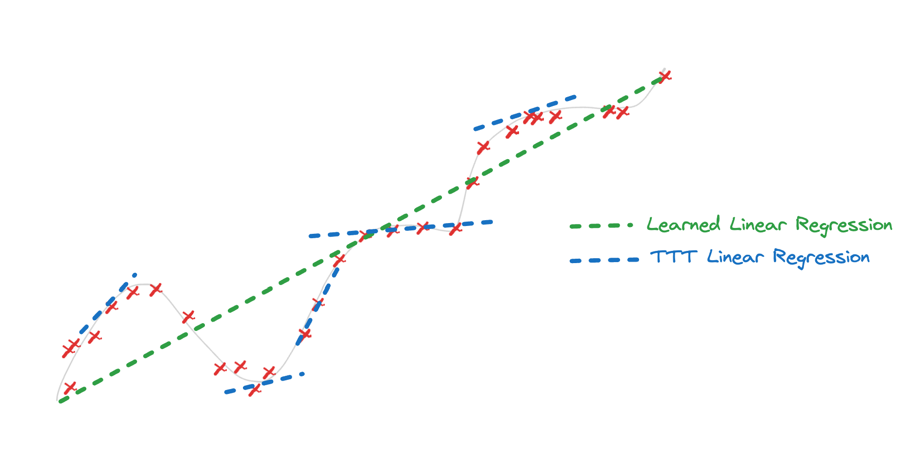
For a simple example, one can take a trained linear regression model, and update the slope for a set of points in the vicinity of the test point and use it make more accurate predictions.
K-Nearest Neighbors is an extreme example of TTT process where the only training that happens is during test time.
In the domain of LLMs, TTT is especially useful, when tasks are complex and outside what an LLM has seen before.
In-Context Learning, few-shot prompting, Chain of Thought reasoning, and Retrieval Augmented Generation have been standards for enhancing LLMs during inference. These techniques enrich context before arriving at a final answer but fail in one aspect—the model is not adapting to the new environment at test time. With TTT, we can make the model learn new concepts that would otherwise needlessly capturing a vast amount of data.

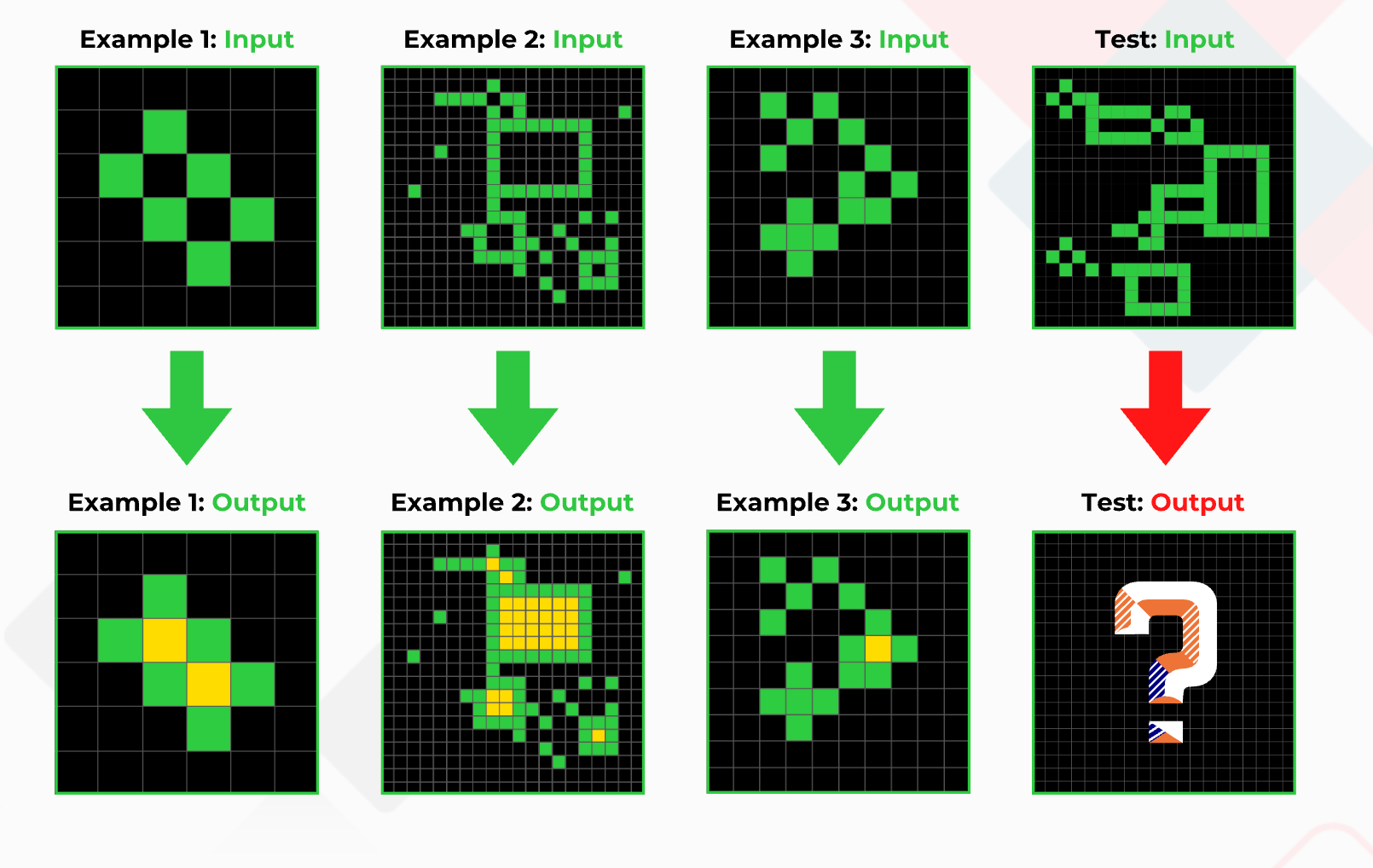
The ARC dataset is an ideal fit for this paradigm, as each data sample is a collection of few-shot examples followed by a question that can only be solved using the given examples—similar to how SAT exams require you to find the next diagram in a sequence.

As shown in the image above, one can use the first three examples for training during the test time and predict on the fourth image.
How to Perform TTT
The brilliance of TTT lies in its simplicity; it extends learning into the test phase. Thus, any standard training techniques are applicable here, but there are practical aspects to consider.
Since training is computationally expensive, TTT adds more overhead since, in theory, you need to train for every inference. To mitigate this cost, consider:
- Parameter-Efficient Fine Tuning (PEFT): During the training of LLMs, training with LoRA is considerably cheaper and faster. Training only on a small subset of layers, like in PEFT, is always advisable instead of full model tuning.
def test_time_train(llm, test_input, nearest_examples, loss_fn, OptimizerClass):
    lora_adapters = initialize_lora(llm)
    optimizer = OptimizerClass(lora_adapters, learning_rate)
    new_model = merge(llm, lora_adapters)

    for nearest_example_input, nearest_example_target in nearest_examples:
        nearest_example_prediction = new_model(nearest_example_input)
        loss = loss_fn(nearest_example_prediction, nearest_example_target)
        optimizer.zero_grad()
        loss.backward()
        optimizer.step()

    predictions = new_model(test_input)
    return predictions
Psuedo-code for test time training with LLMs
- Transfer Learning: During conventional transfer learning, one can replace/add a new task head and train the model
def test_time_train(base_model, test_input, nearest_examples, loss_fn, OptimizerClass):
    new_head = clone(base_model.head)
    optimizer = OptimizerClass(new_head, learning_rate)

    for nearest_example_input, nearest_example_target in nearest_examples:
        nearest_example_feature = base_model.backbone(nearest_example_input)
        nearest_example_prediction = new_head(nearest_example_feature)
        loss = loss_fn(nearest_example_prediction, nearest_example_target)
        optimizer.zero_grad()
        loss.backward()
        optimizer.step()

    test_features = base_model.backbone(test_input)
    predictions = new_head(test_features)
    return predictions
Psuedo-code for test time training with conventional transfer learning
- Embedding Reuse: Track which inferences were made, i.e., which LoRAs were used. During inference, if a new data point’s embedding is close enough to existing ones, an existing LoRA/Task-Head might be reused.
- Test Time Augmentations (TTA): TTA clones the inference image and applies augmentations. The average of all predictions provides a more robust outcome. In TTT, this can improve performance by enriching the training data.
Real-World Uses
- Medical Diagnosis: Fine-tuning general diagnostic models for specific patient conditions or rare diseases with limited data.
- Personalized Education: Adapting an educational AI to a student’s learning style using specific examples.
- Customer Support Chatbots: Enhancing chatbots for niche queries by retraining on specific issues during a session.
- Autonomous Vehicles: Adapting vehicle control models to local traffic patterns.
- Fraud Detection: Specializing models for a specific business or rare transaction patterns.
- Legal Document Analysis: Tailoring models to interpret case-specific legal precedents.
- Creative Content Generation: Personalizing LLMs to generate contextually relevant content, like ads or stories.
- Document Data Extraction: Fine-tuning for specific templates to extract data with higher precision.
Advantages
- Hyper-specialization: Useful for rare data points or unique tasks.
- Data Efficiency: Fine-tuning with minimal data for specific scenarios.
- Flexibility: Improves generalization through multiple specializations.
- Domain Adaptation: Addresses distribution drift during long deployments.
Disadvantages
- Computational Cost: Additional training at inference can be costly.
- Latency: Not suitable for real-time LLM applications with current technology.
- Risk of Poor Adaptation: Fine-tuning on irrelevant examples may degrade performance.
- Risk of Poor Performance on Simple Models: TTT shines when the model has a large number of parameters to learn and the data during test time is of high degree variance. When you try to apply TTT with simple models such as linear regression it will only overfit on the local data and this is nothing more than over-fitting multiple models using KNN sampled data.
- Complex Integration: Requires careful design for integrating training into inference and monitoring multiple models.
TTT is a promising tool, but with significant overhead and risks. When used wisely, it can push model performance in challenging scenarios beyond what conventional methods can achieve.


